Radiation Tutorial
This tutorial will show how to use the radiation support in order to calculate dose-rates and visualise radiation.
The radiation functionality is implemented by sets of compontents that work together. There are components for holding data, components for differect calculation methods and componencts for visualising the result. Seperating the functionality into components provides flexebility at the expense of user friendliness, as there are quite a bit that has to be set up in order to get things up and working.
Calculator
The first thing we will set up is a calculation method. The job of the calculator is to take a cartesion (x,y,z) coordianate as input and provide a dose-rate value back. Three different categories of calculation methods are supported. Interpolation of scattered measurements uses a set of (x,y,z,dose-rate) values as input data and blends one or more of these to give a result back. The point kernel methods uses sources and shields to quickly estimate the simulation of the radiation in order to determine the dose-rate. Finally, the dose map method uses a regular grid of dose-rates and interpolates between the closest points. In this tutorial we will use the simplest scattered measurement method, namely Neareast Neighbor. It will simply find the closest point and return its dose-rate.
From the main menu choose "Add Object" - "Radiation" - "Interpolation" - "Nearest Neighbor"
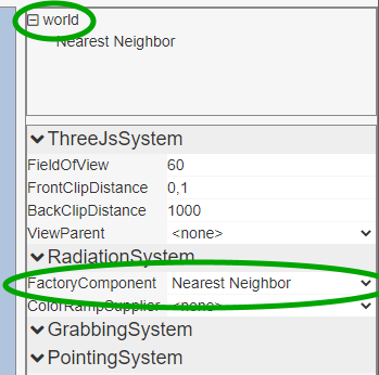
Important: Just adding a calculator does not mean it will automaticly be used by the visualisation components. There can be several calculators in the world but we only want one to be used at a time for consistency. That is why the active calculator is defined by the RadiationSystem. Lets make the Nearest Neighbor calculator the active one.
- Click on the "World" item at the root of the hierarcy pane
- Select Nearest Neighbor as the Factory Component property
Data
The next step is to provide measurements for the Nearest Neighbor calculator. There are currently two componenct that does this. The "CSV Measurement Provider" component reads the measurements from a csv file. The other way, and the one we will use in this tutorial, is to use the "Object Measurment Provider" component. Add it to the world by selecting "Add Object" - "Radiation" - "Interpolation" - "Object Measurment Provider" from the main menu. This component will track all the position and value of all the Measurement components in the world and notify any users when it change.
Add a measurement by selecting "Add Object" - "Radiation" - "Interpolation" - "Measurment" from the main menu. Set the "Value" property to 5. Finally we need tell the Neirest Neighbor calculator to use the Object Measurement Provider. Select the Neirest Neighbor calculator and set the Measurements proprty to Object Measurement Provider.
Dosimeter
Now we want to use the calculator by checking the calculated dose-rate at a certain position. Add a Dosimeter by selecting "Add Object" - "Radiation" - "Dosimeter" from the main menu. The Dosimeters DoseRate property should read 5. If it does not you can follow these troubleshooting tips:
- Check that the radiation server is running.
- Check that the right calculator is selected on the Radiation System.
- Check that that the calculators Measurements property is set to the Object Measurement Provider .
Visualisation
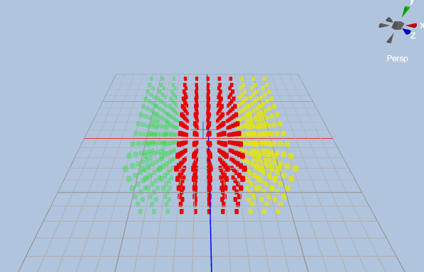
Lets visualise the radiation by having a grid of boxes where each box is colored according to the radiation level. Most of the visualsation methods are based on a 3D grid. That is why we will need to start by adding a visualisation grid component. Select "Add Object" - "Radiation" - "Visualisation" - "Visualisation Grid" from the main menu. The grid defines the bounds of the area we will visualise and the resolution of the grid. Next we will add the Scalar Field Visualisation component. However it depends on the Visualisation Grid component and the dependency is defined as two components haveing to be on the same object. So select the object containing the Visulisation Grid, then select "Add Component" - "Radiation" - "Visualisation" "Scalar Field Visualisation" from the main menu. A grid of red boxes should appear in the 3D view.
To make a slightly more intereseting visualisation add a measurement with value 1 at position (5, 0, 0) and value 0 at (-5, 0, 0). Now the boxes should be colored red, green and yellow. Note that the transforms are relative to the parent so put the measurements at the root of the hierarcy to avoid any transform hierarcy issues.